Acylphosphatase Homologs#
In this tutorial, we shall analyze the molecular dynamics (MD) trajectories of four acylphosphatase (AcP) homologs:
PDB ID |
Organism |
|---|---|
2VH7 |
Human |
2GV1 |
E. coli |
2ACY |
Bovine |
1URR |
Fruit Fly |
Download the data from acylphosphatase.tar.gz
If you are new to running MD simulations using GROMACS, please refer to the legendary GROMACS tutorial Lysozyme in Water by Dr. Justin A. Lemkul at http://www.mdtutorials.com/.
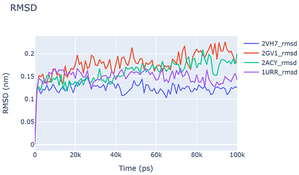
RMSD and RG#
Often the first step after a successful MD simulation is to calculate the root-mean-square deviation (RMSD) and radius of gyration (RG). In GROMACS, these can be calculated using gmx rms and gmx gyrate, respectively.
gmx rms -f 2VH7/2VH7_trajectory.xtc -s 2VH7/2VH7_structure.pdb -o 2VH7/2VH7_rmsd
gmx gyrate -f 2VH7/2VH7_trajectory.xtc -s 2VH7/2VH7_structure.pdb -o 2VH7/2VH7_rg
2VH7_rmsd.xvg and 2VH7_rg.xvg are text files containing the RMSD and RG, respectively. Repeat the process for all the other trajectories.
Note
If you have installed MD DaVis in a virtual or conda environment as suggested in the installation instructions, make sure to activate it before running the md-davis commands.
Plot 2VH7_rmsd.xvg using:
md-davis xvg 2VH7/2VH7_rmsd.xvg -o 2VH7/2VH7_rmsd.html
You should obtain a plot like this:
To plot the RMSD from the four trajectories together, use:
md-davis xvg 2VH7/2VH7_rmsd.xvg 2GV1/2GV1_rmsd.xvg 2ACY/2ACY_rmsd.xvg 1URR/1URR_rmsd.xvg -o AcP_rmsd.html
Similarly, the RG can also be plotted using the md-davis xvg command.
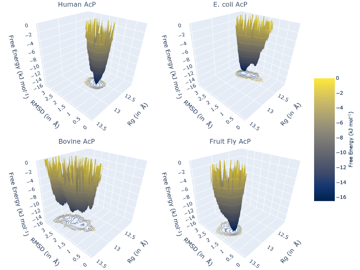
Create Free Energy Landscapes#
Next, we will create the free energy landscape using RMSD and RG as the x and y variables. The sample trajectories provided with this tutorial only contain 100 frames to keep their sizes small. Thus, the RMSD and RG files created at the beginning of this tutorial only contain 100 timesteps each. Using 100 points to create a free energy landscape would not be accurate. Therefore, the RMSD and RG files calculated from the full 1 μs trajectory containing 100,000 frames are provided with the tutorial. Use these files to create the free energy landscape. For human acylphosphatase, the free energy landscape can be created with:
md-davis landscape_xvg -T 300 -x 2VH7/2VH7_rmsd_full.xvg -y 2VH7/2VH7_rg_full.xvg -n "2VH7" -l "Human AcP" -o 2VH7_landscape.html
Here, -T 300 specifies 300 K as the temperature of the system. Now to plot all four landscapes together:
md-davis landscape_xvg -T 300 --common -x 2VH7/2VH7_rmsd_full.xvg -y 2VH7/2VH7_rg_full.xvg --name "2VH7" --label "Human AcP" -x 2GV1/2GV1_rmsd_full.xvg -y 2GV1/2GV1_rg_full.xvg --name "2GV1" --label "E. coli AcP" -x 2ACY/2ACY_rmsd_full.xvg -y 2ACY/2ACY_rg_full.xvg --name "2ACY" --label "Bovine AcP" -x 1URR/1URR_rmsd_full.xvg -y 1URR/1URR_rg_full.xvg --name "1URR" --label "Fruit Fly AcP" -o AcP_FEL.html
In the command above, remember to provide -x, -y, --name, and --label together before those for the subsequent trajectory. The option --common instructs MD DaVis to create the four landscapes using identical ranges and binning, which allows us to compare the landscapes reliably. The output from the above command is shown below; click the image to view the interactive HTML file.
Electrostatic Potential and Electric Field Dynamics#
Create a sample of frames for calculating the electrostatic potential with DelPhi
mkdir 2VH7/2VH7_electrostatics/
gmx trjconv -f 2VH7/2VH7_trajectory.xtc -s 2VH7/2VH7_structure.pdb -o 2VH7/2VH7_electrostatics/2VH7_frame.pdb -dt 10000 -sep
MD DaVis has the
electrostaticscommand, which is a wrapper for running DelPhi and reporting the electrostatic potential at the vertices of a triangulated surface obtained using MSMS
md-davis electrostatics --surface -m ~/msms_i86_64Linux2_2.6.1/msms.x86_64Linux2.2.6.1 -d ~/delphicpp_v8.4.5_serial -o 2VH7/2VH7_electrostatics/ 2VH7/2VH7_electrostatics/2VH7_frame*.pdb
In the command above, the MSMS directory and the DelPhi executable are placed in the home folder. Adjust the path according to your system.
The electrostatic potential on the surface and the dynamics of the electric field around the molecule can be visualized with the following command:
md-davis electrodynamics --ss_color --surface --name Human_AcP 2VH7/2VH7_electrostatics
Residue Properties Plot#
Calculate the root-mean-square fluctuation, solvent accessible surface area, and secondary structure using GROMACS:
gmx rmsf -res -f 2VH7/2VH7_trajectory.xtc -s 2VH7/2VH7_structure.pdb -o 2VH7/2VH7_rmsf
gmx sasa -f 2VH7/2VH7_trajectory.xtc -s 2VH7/2VH7_structure.pdb -o 2VH7/2VH7_sasa.xvg -or 2VH7/2VH7_resarea.xvg
gmx do_dssp -f 2VH7/2VH7_trajectory.xtc -s 2VH7/2VH7_structure.pdb -o 2VH7/2VH7_dssp -ssdump 2VH7/2VH7_dssp -sc 2VH7/2VH7_dssp_count
Repeat for the remaining trajectories. We will also plot the torsional flexibility, but that will be calculated by MD DaVis later.
Note
For the gmx do_dssp command to work, the dssp or mkdssp binary must be available on your system. Download it from ftp://ftp.cmbi.ru.nl/pub/software/dssp/ and ensure GROMACS can find it by setting the DSSP environment variable to point to its location on your system.
Collect and store all the calculated properties into an HDF file. To do that, first, create a TOML file as shown below, telling MD DaVis the location of each file.
name = '2VH7'
output = '2VH7_data.h5'
label = 'Human AcP'
text_label = 'Human AcP'

trajectory = '2VH7_trajectory.xtc'
structure = '2VH7_structure.pdb'

[timeseries]
    rmsd = '2VH7_rmsd_full.xvg'
    rg = '2VH7_rg_full.xvg'

[dihedral]
    chunk = 101

[residue_property]
    secondary_structure = '2VH7_dssp.dat'
    rmsf = '2VH7_rmsf.xvg'
    sasa = '2VH7_resarea.xvg'
    surface_potential = '2VH7_electrostatics'   # directory containing electrostatic calculations
Input TOML file for each trajectory is provided with the tutorial files. Next, collate all the data using MD DaVis, which can process multiple TOML files and create the respective HDF file.
md-davis collate 2VH7/2VH7_input.toml 2GV1/2GV1_input.toml 2ACY/2ACY_input.toml 1URR/1URR_input.toml
Combine the data from the HDF file into a pandas dataframe with:
md-davis residue 2VH7_data.h5 2GV1_data.h5 2ACY_data.h5 1URR_data.h5 -o AcP_residue_data.p
Plot the residue properties:
md-davis plot_residue AcP_residue_data.p -o AcP_residue_data.html
Now, we can also align the residues of the different trajectories to align the peaks in the data.
obtain the sequence of residues in FASTA format from each PDB file using the
sequencecommand in MD DaVis:
md-davis sequence 2VH7/2VH7_structure.pdb -r fasta
Use a sequence alignment program or webservers like Clustal Omega or T-coffee to obtain the alignment of these sequences in ClustalW format.
CLUSTAL O(1.2.4) multiple sequence alignment


2GV1_structure      ---MSKVCIIAWVYGRVQGVGFRYTTQYEAKRLGLTGYAKNLDDGSVEVVACGEEGQVEK    57
1URR_structure      -VAKQIFALDFEIFGRVQGVFFRKHTSHEAKRLGVRGWCMNTRDGTVKGQLEAPMMNLME    59
2VH7_structure      ----TLISVDYEIFGKVQGVFFRKHTQAEGKKLGLVGWVQNTDRGTVQGQLQGPISKVRH    56
2ACY_structure      AEGDTLISVDYEIFGKVQGVFFRKYTQAEGKKLGLVGWVQNTDQGTVQGQLQGPASKVRH    60
                          ..:   ::*:**** **  *. *.*:**: *:  *   *:*:    .   :: .

2GV1_structure      LMQWLKSGGPRSARVERVLSEPH--HPSGELTDFRIR-  92
1URR_structure      MKHWLENNRIPNAKVSKAEFSQIQEIEDYTFTSFDIKH  97
2VH7_structure      MQEWLETRGSPKSHIDKANFNNEKVILKLDYSDFQIVK  94
2ACY_structure      MQEWLETKGSPKSHIDRASFHNEKVIVKLDYTDFQIVK  98
                    : .**:.    .:::.:.         .   :.* *
Create a TOML file to specify which alignment file corresponds to which chain and which sequence label corresponds to which data, as shown below:
[names]
2GV1 = '2GV1_structure'
1URR = '1URR_structure'
2VH7 = '2VH7_structure'
2ACY = '2ACY_structure'

[alignment]
'chain 0' = 'AcP_alingment.clustal_num'
Run the
md-davis residuecommand passing the TOML file with the--alignmentoption to generate the pandas dataframes.
md-davis residue 2VH7_data.h5 2GV1_data.h5 2ACY_data.h5 1URR_data.h5 --alignment Acp_alignment_input.toml -o AcP_residue_data_aligned.p
Plot the aligned data frames.
md-davis plot_residue AcP_residue_data_aligned.p -o AcP_residue_data_aligned.html
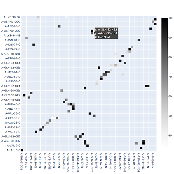
Hydrogen Bond Matrix#
Calculate the hydrogen bonds using the
hbondutility in GROMACS.
gmx hbond -f 2VH7/2VH7_trajectory.xtc -s 2VH7/2VH7_md.tpr -num 2VH7/2VH7_hbnum.xvg -hbm 2VH7/2VH7_hb_matrix -hbn 2VH7/2VH7_hb_index
2. Open the output index file 2VH7_hb_index.ndx and scroll down to find the
title of the last section containing the list of hydrogen bonds, which is hbonds_Protein in this case, as shown below:
 1235  1243  1244  1248  1249  1260  1261  1263  1264  1280  1285  1286  1301  1302  1320
 1321  1339  1340  1356  1361  1362  1380  1381  1389  1390  1392  1393  1410  1413  1414
 1421  1424  1425  1433  1434  1436  1437  1456  1457  1468  1469  1473  1474  1492  1493
 1508  1509  1525  1530  1531
[ hbonds_Protein ]
      9     10     35
     36     37    773
     55     56   1285
     62     63    725
Calculate the occurrence of each hydrogen bond:
md-davis hbond -x 2VH7/2VH7_hb_matrix.xpm -i 2VH7/2VH7_hb_index.ndx -s 2VH7/2VH7_structure.pdb -g hbonds_Protein --save_pickle 2VH7/2VH7_hbonds.p
Plot the hydrogen bonds matrix
md-davis plot_hbond --percent --total_frames 101 --cutoff 33 -o 2VH7_hbond_matrix.html 2VH7/2VH7_hbonds.p
The above command plots the percentage of the H-bonds, which is calculated for each H-bond as follows:
number of frames the H-bond is observed / total number of frames * 100
The cutoff of 33 % is set to plot only those H-bonds whose occurrence is greater than 33 %.