Surface Electrostatic Potential Per Residue

Usually, the distribution of electrostatic potential around a protein molecule is visualized by solving the Poisson-Boltzmann equation using a grid base approach (APBS/Delphi) and coloring the molecular surface with the obtained electrostatic potentials, as shown below.

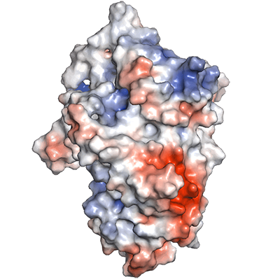
This only allows for qualitative inspection of one structure or conformation at a time. In contrast, MD DaVis can calculate the surface electrostatic potential per residue from electrostatics calculations on a sample of conformation from the MD trajectory. Thereby, incorporating dynamical information into the analysis. The steps involved are as follows:

1. Obtain a sample of conformations from the trajectory as PDB files. Ideally, all the conformations should be centered at the origin and aligned. Optionally, the reference conformation used for alignment may be oriented with its first, second and third principal axis along the x, y, and z axis, respectively. When comparing samples from two or more trajectories ensure that the reference structures for each are aligned to reduce discrepancy caused by grid selection during electrostatics calculation.

2. Use md-davis electrostatics to run MSMS and DelPhi on each PDB file.

   md-davis electrostatics --surface -m <MSMS> -d <DELPHI> -o <OUTPUT_DIR> [PDB_FILES]
   

   This calculates the triangulated molecular surface using the MSMS program (Sanner et al., 1996) and evaluates the electrostatic potentials at the vertices of the triangulated surface using Delphi (Li et al., 2019). In addition, the volumetric data for electrostatic potential at grid points around the molecule are also saved by DelPhi in Gaussian CUBE format. This can be used for 3D vislization of the surface electrostatic potentials (Figure above) or electric field dynamics. It is advisable to align the PDB files and specify the grid size for Delphi calculation, so that the same grid points are used for each calculation.

3. Specify the path to the directory containing the surface potential files in the input TOML file used by :ref:`collate.

   [residue_property]
       surface_potential = '<OUTPUT_DIR>'
   

4. The total and mean electrostatic potential per residue is calculated when the data is collated into an HDF file.

   md-davis collate input.toml
   

   This will search for all .pot files in the specified <OUTPUT_DIRECTORY>. The vertices corresponding to each residue are identified along with the corresponding electrostatic potential. The total and mean of the electrostatic potentials on the vertices for each residue are calculated. The total gives information about the charge on the surface as well as the exposed surface area, while the mean nullifies the contribution from the exposed surface area. The mean and standard deviation of both are calculated and saved in the output HDF file.

5. Follow the steps for creating a residue property plot to visualize the data.

   md-davis plot residue output_residue_wise_data.p
   

Note

A discrepancy between the molecular surface calculated by MSMS and the molecular surface used by DelPhi to detect the protein’s interior was observed for buried residues in multimeric proteins. DelPhi uses a different dielectric constant for the molecule’s interior, so the potential on these residues was very high.

md-davis electrostatics --surface -m <MSMS_EXECUTABLE> -d <DELPHI_EXECUTABLE> -o <OUTPUT_DIRECTORY> [PDB_FILES]

md-davis electrostatics is a wrapper for running Delphi and reporting the electrostatic potential at the vertices of a triangulated surface obtained using MSMS. Therefore, these must be installed for this command to work, which may be downloaded from http://compbio.clemson.edu/delphi and http://mgltools.scripps.edu/downloads#msms, respectively.

The default parameters used for running Delphi are:

• 2000 linear interations

• maximum change in potential of 10^-10 kT/e.

• The salt concentration is set to 0.15 M

• solvent dielectric value of 80 (dielectric of water)

If you want to use different set of parameters, you may run Delphi without the md

The atomic charges and radii from the CHARMM force field are provided by default. The parameter files containing the atomic charges and radii for DelPhi are available at: http://compbio.clemson.edu/downloadDir/delphi/parameters.tar.gz

The output potential map is saved in the cube file format (used by Gaussian software); the other formats do not load in molecular visualization software.

The following charge and radius files are provided with the source code for MD DaVis.

md_davis/md_davis/electrostatics/charmm.crg md_davis/md_davis/electrostatics/charmm.siz

If you receive a warning during Delphi run regarding missing charge or radius. Then the missing properties must be added to these files or whichever files you provide to md-davis electrostatics.

Electric Field Dynamics

The electrostatic potentials calculated in Surface Electrostatic Potential Per Residue can be visualized as a 3D animation of electric field lines using:

md-davis electrodynamics --ss_color --surface --name Human_AcP 2VH7/2VH7_electrostatics

This creates a PyMOL session with the conformations as frames in the animation as shown below:

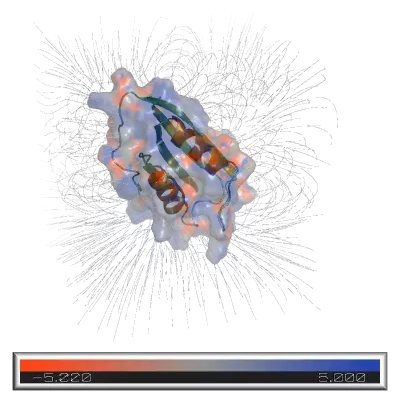
1. The coordinates of the reference structure are translated to place the center of mass of the molecule at the origin and rotated so that the first, second, and third principal axes are along the x, y, and z-axes, respectively.

2. The frames sampled from the trajectory are aligned to the reference.

3. The electrostatic potentials are obtained for each sampled structure using Delphi. The box for each calculation is centered at the origin, and the number of grid points is manually set to the same value for each structure to ensure the same box size during each calculation.

4. The surface electrostatic potentials calculated per residue or atom are written into the output PDB file’s B-factor or occupancy column.

5. The output PDB file and the corresponding electric field from the sample are visualized as frames in PyMOL (Schrödinger, LLC, 2015), which can animate the dynamics of the electric field lines.