Free Energy Landscapes#
The free energy landscape of a protein is a continuous function between the protein conformations and the free energy. MD DaVis creates free energy landscapes using the method described in Tavernelli et al., 2003. First, the user must provide two quantities of interest to classify the protein conformations, such as root mean square deviation (RMSD) and radius of gyration (RG), or the projection on the first two eigenvectors from principal component analysis. Then, the two variables are binned to make a 2D histogram, and the free energy landscape is obtained by Boltzmann inversion of the histogram using:
where, \(\Delta \varepsilon_i\) is the change in free energy between the conformations in the ith bin and the maximally occupied bin, \(n_i\) and \(n_{max}\) are the number of conformations in these, respectively. This formula results in 0 energy for the most probable state and all other states having positive energy. Since the absolute free energy is impossible to calculate and only the change in free energy is meaningful, the maximum value in the free energy landscape is subtracted from all the bins so that the most probable state has the most negative free energy.
The interactive 3D plot of the free energy landscape can be rotated and viewed from various directions, zoomed in and out, and labels on the surface inspected to determine the valleys and wells.
A unique feature of MD DaVis is that rotating one landscape in a plot with multiple landscapes rotates all to the same view.
The trajectory points can also be animated or plotted on top of the free energy landscape; this allows inspecting the traversal of wells in the free energy landscapes during the MD simulation.
The landscapes can be plotted using common ranges and same number of bins, enabling their comparison. The wonderful feature of the plot created using MD DaVis is that it is an interactive html, and rotating one subplot rotates all others to the same view. These features facilitate the quick and efficient comparison of the free energy landscapes.
Note
Plotting free energy landscapes requires a large number of frames, therefore, always save enough number of frames during the simulation. The number of frames required to obtain a reasonable representation of the free energy landscape depends on flexibility of the protein. If the protein accesses a large number of conformational states a greater number of frames would be required. As a ball park, at least 10000 frames are required.
Note
These commands do not open the output html file in a web browser like other plotting commands, so please check the working directory for the output html file. If a file with the same name exists, it will be overwritten.
Free Energy Landscapes from xvg files#
The quickest way to plot the free energy landscape is from text files containing the two properties of interest.
md-davis landscape_xvg -c -T 300 -x rmsd_1.xvg -y rg_1.xvg -n "name_1" -l "FEL for 1"
Here, .xvg the file containing the RMSD and RG
precalculated using GROMACS is provided as the -x and -y input files.
While providing other properties or files not created by GROMACS ensure that they are two column files
If the output filename is not provided the default name is landscape.html.
-c specifies that the ranges of the all the landscapes must be the same
-T 300 specifies to use 300 K as the temperature for the boltzmann
inversion. If this option is not provided, only the 2D histrogram of the
data is plotted.
An excellent feature of MD DaVis is that while creating the 2D histogram, it creates a data structure in which the index of each frame in a particular bin is stored. This feature allows one to find the frames in a particular bin of the landscape, and the frames in the minima are generally of particular interest.
To plot multiple free energy landscapes as subplots just provide the inputs one after the other. The -x, -y, -n, and -l for one trajectory must be provided together before the next set of inputs from the other trajectory.
md-davis landscape_xvg -c -T 300 -x rmsd_file_1.xvg -y rg_file_1.xvg -n "name_1" -l "Free Energy Landscape for 1" -x rmsd_file_1.xvg -y rg_file_1.xvg -n "name_2" -l "Free Energy Landscape for 2" -x rmsd_file_1.xvg -y rg_file_1.xvg -n "name_3" -l "Free Energy Landscape for 3"
Plot Free Energy Landscapes from HDF Files#
If the RMSD and RGhave been collated into HDF files for each trajectory. These may be plotted using:
md-davis landscape rmsd_rg -c -T 300 file1.h5 file2.h5 file3.h5
Plot Free Energy Landscapes Overlaid with Trajectory Points#
One must save the landscape created by landscape_xvg or landscape with the -s option before this one can be used. Since the output generated for single landscape is big, visualization of multiple landscapes becomes impractical. So, it only plots one landscape at a time. Select the desired landscape in landscapes.h5 by providing its index with -i. By default only the first landscape is plotted
md-davis landscape animation landscapes.h5 -i 0 --static -o trajectory.html
## Step 4: Free energy Landscapes
### Create and plot free energy landscapes using common bins and ranges
md-davis landscape rmsd_rg -T 300 --common --select backbone output1.h5 output2.h5 -s landscapes.h5
This command will create an html file with the interactive landscapes. It will not open the file like other plotting commands, so check the working directory for the output html file.
### Plot free energy landscape overlaid with trajectory points
One must save the landscape created by the previous command with -s before this one can be used. Since the output generated for single landscape is big, visualization of multiple landscapes becomes impractical. So, it only plots one landscape at a time. Select the desired landscape in landscapes.h5 by providing its index with -i. By default only the first landscape is plotted
md-davis landscape animation landscapes.h5 -i 0 --static -o trajectory.html
Note
The first rotation may not sync across all subplots. Please rotate again to sync the view of all the subplots. Also, zooming a subplot is also not synchronized immediately. After zooming a subplot rotate the same subplot to sync the zoom on all subplots.
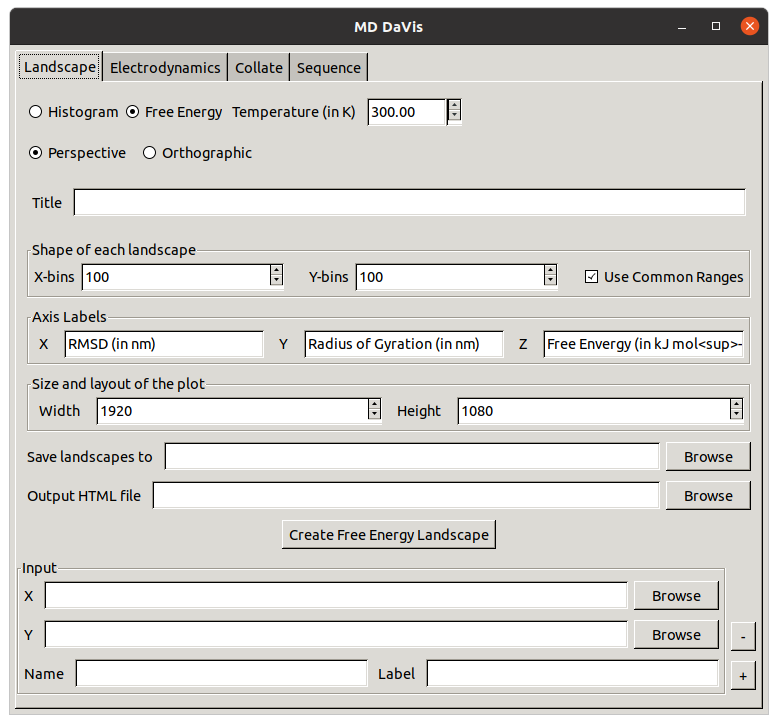
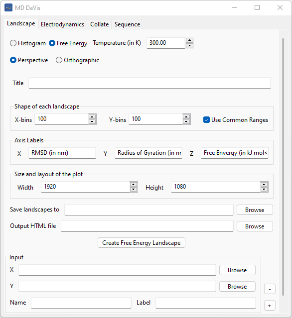
Plot Free Energy Landscapes using the MD DaVis GUI#
The free energy landscapes from xvg files can also be created using the Landscape tab in the MD DaVis GUI. Plotting from HDF files and animated/overlaid trajectories is not supported using the GUI but shall be incorporated soon.