Quickstart#
The following steps walks you through the process of using the MD DaVis graphical user interface (GUI) and command line interface (CLI) to assimilate the analysis data and creating interactive plots.
Step 1: Calculate the required quantities#
MD DaVis has been designed to natively work with the output from GROMACS analysis tools. However, the same analysis performed with other tools may be visualized by MD DaVis as long as the input files can be be appropriately formatted. Root mean squared deviation (RMSD) and radius of gyration (RG) will be used to create free energy landscapes and the rest will be used for residue property plot. Ensure that the trajectories and structures are processed and corrected for periodic boundary conditions.
Root mean squared deviation (RMSD)#
gmx rms -f trajectory.trr -s structure.pdb -o rmsd.xvg
The structure provided will be used as the reference for calculating RMSD of the trajectory.
Radius of gyration (RG)#
gmx gyrate -f trajectory.trr -s structure.pdb -o rg.xvg
Root mean squared fluctuation (RMSF)#
gmx rmsf -f trajectory.trr -s structure.pdb -res -o rmsf.xvg
This would use the whole molecule for RMSF calculation. You may calculate the RMSF of each chain separately in a protein with multiple chains. This would reflect the fluctuations only due to backbone motion and eliminate the fluctuation from relative motion of chains.
Solvent accessible surface area (SASA)#
To calculate the average SASA per residue pass -or option to gmx sasa.
gmx sasa -f trajectory.trr -s structure.pdb -o sasa.xvg -or resarea.xvg
Secondary structure using DSSP#
gmx do_dssp -f trajectory.trr -s structure.pdb -o dssp -ssdump sec_str -sc sec_str_count
Step 2: Collate the data into an HDF file#
Use the collate tab in the MD DaVis GUI
to collect all the analysis data calculated above into a HDF file (data.h5)
for organized storage and input to subsequent commands.
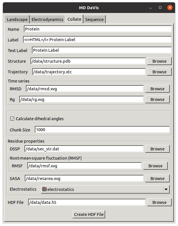
According to the image the files calculated in Step 1 are in /data
directory.
See the collate user guide page for more details.
Step 3: Plot the free energy landscape#
You can directly plot the free energy landscape from the RMSD and Rg files
using the md-davis landscape_xvg command or the GUI as shown below:
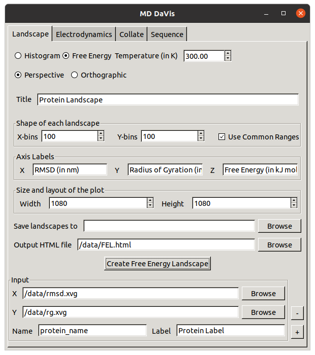
This will create a free energy landscape like the image shown below; click the image to open the interactive HTML plot.
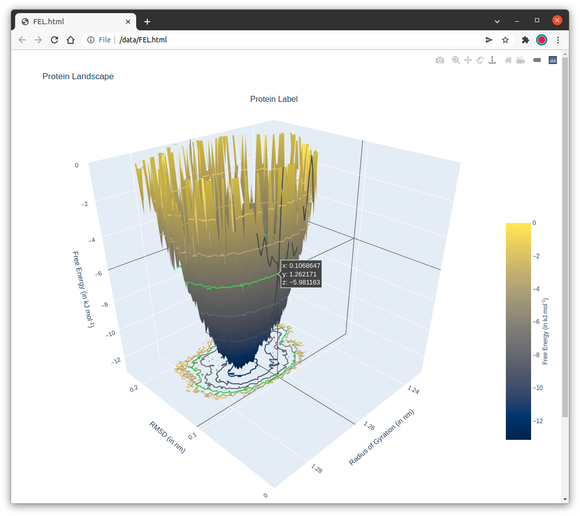
Or, you can plot the free energy landscape from the HDF file created in Step 2.
md-davis landscape -T 300 --common data.h5 -o FEL.html
This command will create the FEL.html file with the interactive landscape. It will not open the file like other plotting commands, so check the working directory for the output html file.
Step 4: Plot the residue property plot#
Step 4a: Create a pickle file (a serialized binary file used to store python objects) with the residue dataframe using:
md-davis residue data.h5 -o residue_dataframe.p
Step 4b: Plot the pickle file from the previous command using:
md-davis plot_residue residue_dataframe.p -o plot.html